Energy Management of PV-Battery Systems for Rural Microgrids and Agricultural Water Pumping Applications in Senegal

Souleymane Soumah; Mouhamadou Falilou Ndiaye; Mohamed Ansoumane Camara; Vincent Sambou

doi:doi:10.11648/j.sjee.20251304.12

Research Article |

| Peer-Reviewed

Energy Management of PV-Battery Systems for Rural Microgrids and Agricultural Water Pumping Applications in Senegal

Souleymane Soumah^*

, Mouhamadou Falilou Ndiaye

, Mohamed Ansoumane Camara

, Vincent Sambou

Published in Science Journal of Energy Engineering (Volume 13, Issue 4)

Received: 10 November 2025 Accepted: 21 November 2025 Published: 17 December 2025

Views: Downloads:

Download PDF

Share This Article

Twitter
Linked In
Facebook

Abstract

This work proposes an optimized energy management strategy for a photovoltaic (PV) system coupled with batteries, intended for both rural electrification and agricultural pumping applications. The approach takes into account photovoltaic generation, battery storage and demand management to ensure a balance between domestic needs and irrigation requirements. For the MPPT of PVs with an installed power of 36.6 kWp, we used the conductance increment algorithm (Inc) to provide the PV current reference and the power transfer to the DC bus was provided via a Boost chopper. To ensure the stability of the DC bus voltage, a PI regulator is dimensioned and a management algorithm is developed to control the Buck-Boost coupled to the grid. This algorithm makes it possible to store the excess PV production in the battery pack and to return them in the event of a deficit through the bidirectional converter. In addition, the proposed strategy ensures coordinated operation between generation, storage, and agricultural pumping in order to guarantee the continuity of supply under varying climatic and load conditions. The simulation results highlight the potential of PV-battery microgrids to reduce reliance on diesel, improve access to water for agriculture, and strengthen the sustainability of rural communities. The findings demonstrate that the proposed system achieves stable voltage regulation, efficient energy allocation, and improved autonomy for isolated sites. The study thus proposes a framework that can be replicated in similar contexts in sub-Saharan Africa, simultaneously contributing to energy access and food security.

Published in	Science Journal of Energy Engineering (Volume 13, Issue 4)
DOI	10.11648/j.sjee.20251304.12
Page(s)	192-205
Creative Commons	This is an Open Access article, distributed under the terms of the Creative Commons Attribution 4.0 International License (http://creativecommons.org/licenses/by/4.0/), which permits unrestricted use, distribution and reproduction in any medium or format, provided the original work is properly cited.
Copyright	Copyright © The Author(s), 2025. Published by Science Publishing Group

Keywords

Energy Management, MPPT, Photovoltaic Systems, Battery Storage, Agricultural Pumping, Microgrids

1. Introduction

Rural electrification in developing countries remains a major challenge for achieving the Sustainable Development Goals

[1]

. Despite abundant energy resources (solar, biomass, hydroelectricity), access remains unequal between urban and rural areas

[2]

. Despite the efforts of governments, a large part of the rural population in these countries still does not have access to electricity

[3]

. In 2015, the rural electrification rate in Senegal did not exceed 30%

[4]

, Faced with this reality, photovoltaic (PV) systems combined with battery storage appear to be a favourable alternative to meet the energy needs of these localities

[5]

, These systems not only provide a sustainable alternative to fossil fuel-powered generators, but also help improve the quality of life in communities by promoting lighting, education, health and the development of income-generating activities

[6]

, In the agricultural context, solar energy occupies a strategic place: it makes it possible to pump water for irrigation, to transform and preserve products, and to support new practices that are more resilient to the effects of climate change

[7]

In addition, several studies have shown that microgrids, whether direct current (DC), alternating current (AC) or hybrid, can be adapted to local realities and offer technical and economic viability

[8]

, In their study, Molu and al. developed an energy management system based on linear optimization for a grid-connected PV/battery microgrid, aiming to minimize operating costs over 24 hours. They compared this approach to a heuristic method, demonstrating a reduction in costs, especially in variable weather conditions

[9]

, In Senegal, Cisse and al. developed an energy management strategy for a farm located in Gandon, combining photovoltaic, wind and battery pumping, with modulation of the pump's power and use of the reservoir as hydraulic storage. Their approach covers 100% of water needs while reducing battery usage time by 13%

[10]

, In other studies, Rumbayan and al. designed and tested an innovative system that combines photovoltaic pumping and smart water management via IoT, to ensure a sustainable domestic water supply for rural communities in the North Sulawesi province of Indonesia

[11]

, While Sayani and al. evaluated two strategies for sizing solar mini-grids in rural Indian villages, integrating scenarios of electricity demand growth over ten years. Their analysis shows that a modular approach would save up to 12% compared to a single installation

[12]

In contrast, Kyriakarakos and al.'s research proposed an innovative model of rural electrification in sub-Saharan Africa, based on the investment of agricultural cooperatives in solar microgrids. Using a case study in Rwanda, they simulated different technical and economic scenarios using the HOMER software, comparing configurations with and without productive load (maize mill), to assess the financial viability and cross-subsidy potential for household electrification

[13]

This article analyzes the energy management of PV-battery systems in rural microgrids, with a focus on agricultural applications in Gandon, Senegal. The aim is to develop a strategy to feed irrigation pumps and related loads while ensuring a stable supply and maximising socio-economic and environmental benefits for the local community.

2. Materials and Methods

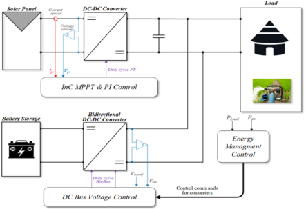
The proposed system (Figure 1), is a direct current microgrid consisting of a photovoltaic array, battery storage and an energy management unit for the simultaneous supply of domestic and agricultural loads. Solar energy is converted via a DC-DC converter controlled by an MPPT conductance increment algorithm, combined with a PI controller, to ensure maximum power extraction. The DC bus, stabilized by capacitive filtering, is the common point of interconnection between the photovoltaic source, the battery and the loads. The storage is coupled to the bus through a bidirectional DC-DC converter, allowing charging in the event of a photovoltaic surplus and discharging when production is insufficient. The voltage regulation of the bus is achieved by a control loop with the PI regulator, ensuring the stability of the system. Finally, an energy management strategy oversees the dynamic distribution of power between source, storage and loads, ensuring continuity of power and optimising the use of available resources.

Download: Download full-size image

Figure 1. Synoptic diagram of the system studied.

Component Modeling

In this part, the modeling of the different components of the microgrid is presented. The mathematical equations describing the photovoltaic source, the storage device, the converters and the loads are presented in order to faithfully represent the overall behavior of the system.

2.1. Module PV

The current flowing through a

p - n

junction (or an equivalent diode in a photovoltaic cell) is described by the following exponential equation

[14, 15]

I_{d} = I_{0} [\exp (\frac{V_{d}}{V_{T}}) - 1]

(1)

The thermal tension is given by:

V_{T} = \frac{kT}{q} \times nI \times Ncell

(2)

Where:

I_{d}

: Diode current (A)

V_{d}

: Diode voltage (V)

I_{0}

: Diode saturation current (A)

nI

: Diode ideality factor, a number close to 1.0

k

: Boltzman constant= 1.3806e-23 J.K^-1

q :

Electron charge= 1.6022e-¹⁹ C

T

: Cell temperature (K)

Ncell

: Number of cells connected in series in a module. This relationship, known as the Shockley equation, reflects the nonlinear behavior of the diode. At low voltages, the current remains close to

, {- I}_{0}

, while at high direct polarization, it increases exponentially. In the case of solar cells, this model is fundamental to describe the current-voltage (I-V) characteristic of the photovoltaic array and serves as a basis for the electrical modeling of the modules.

Overview of photovoltaic parameters

In order to accurately characterize the electrical behavior of the photovoltaic module studied, the main parameters are summarized in Table 1. These parameters, provided by the manufacturer under standard test conditions (STC: 1000 W/m², AM 1.5 spectrum and 25°C cell temperature), are essential for the modeling and evaluation of PV system performance. They include short-circuit current (

I_{sc}

), open-circuit voltage (

V_{oc}

), current (

I_{mpp}

) and voltage (

V_{mpp}

) at the point of maximum power, maximum power delivery (

P_{\max}

), and temperature coefficients of current and voltage. These quantities form the basis of simulation models and allow a consistent comparison between different photovoltaic technologies.

Table 1. PV parameters.

Module	Advance Solar Hydro Wind Power API-150
Maximum Power (W)	150.075
Cells per module (Ncell)	72
Open circuit voltage Voc (V)	41.8
Short-circuit current Isc (A)	5.05
Voltage at maximum power point Vmp (V)	34.5
Current at maximum power point Imp (A)	4.35
Temperature coefficient of Voc (%/deg.C)	-0.419
Temperature coefficient of Isc (%/deg.C)	0.096

2.2. Modeling of the Battery Energy Storage Chain

(i). Storage Battery

The battery's state of charge (SoC), expressed as a percentage, is defined as follows

[16, 17]

{SoC}_{bat} = 100 \times (1 + \frac{1}{Q_{bat}} \times \int_{0}^{t} i_{bat} (t) dt)

(3)

where:

{SoC}_{bat} :

is the state of charge at time t (%),

Q_{bat} :

is the nominal capacity of the battery (Ah),

i_{bat} :

is the current of the battery at time t (A), considered positive in discharge.

This expression is based on the assumption that the battery is initially fully charged (SoC=100% at t=0). The SoC decreases as the battery drains (

i_{bat}

> 0) and increases when recharged (

i_{bat}

< 0). The state of charge (soc) of a battery is the level of charge in relation to its capacity.

The dynamic behavior of the voltage across a battery can be represented by a semi-empirical model integrating ohmic effects, polarization, and internal dynamical phenomena. The instantaneous voltage (

V_{bat})

given by the following expression

[17-20]

V_{bat} = E_{0} - K \times \frac{Q}{Q - i_{t}} - R_{b} \times i + A_{b} \times e^{- B \times i_{t}} - K \times \frac{Q}{Q - i_{t}} \times if

(4)

where:

V_{bat} :

is the instantaneous voltage of the battery (V),

E_{0}

: is the open-circuit electromotive voltage (EMF),

K

: is a polarization coefficient (V),

Q :

is the maximum battery capacity (Ah),

i_{t}

: is the cumulative capacity extracted from the initial instant (Ah),

R_{b}

: is the internal resistance of the battery (Ω),

i :

is the instantaneous current supplied by the battery (A),

A_{b}

and

B :

are constants associated with nonlinear dynamic behavior,

if :

is a conditional indicator factor (e.g., 1 in discharge and 0 in charge or vice versa).

This model allows you to take into account:

The ohmic voltage drop via the term,

R_{b} \times i

Voltage loss due to polarization, modeled by the term

K \times \frac{Q}{Q - i_{t}}

A relaxation or transient response effect via the exponential term

A_{b} \times e^{- B \times i_{t}}

as well as an additional conditional adjustment by the last term.

In order to preserve battery life and ensure safe operation, the SoC is constrained within a permissible range defined by

[20]

{SoC}_{batmin} \leq {SoC}_{bat} \leq {SoC}_{batmax}

(5)

Where:

{SoC}_{batmin}

: corresponds to the maximum permitted depth of discharge,

{SoC}_{batmax}

: is the maximum load level allowed.

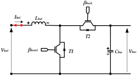
(ii). Topologie du Convertisseur DC–DC Bidirectionnel

Figure 2 shows a non-isolated bidirectional DC–DC converter that interfaces between the battery (

V_{bat}

) and the DC bus (

V_{bus}

). The structure consists of a series inductor

L_{b}

, two controlled switches (βboost and βbuck) associated with their anti-parallel diodes (

T_{1}

T_{2}

), and a capacitor

C_{bus}

that stabilises the bus voltage.

In boost mode (battery discharge), the βboost switch modulates the current

i_{bat}

in the inductance, allowing energy to be transferred to the bus via the diode

T_{2}

. In buck mode (battery charge), βbuck controls the transfer of energy from the bus to the inductance and battery, while

T_{1}

provides a free path for the current to flow.

This bidirectional topology ensures efficient energy exchange between the storage element and the DC bus, making it particularly suitable for PV systems and hybrid microgrids.

Download: Download full-size image

Figure 2. Buck-Boost bidirectional DC‐DC converter

[21]

The model of the bidirectional converter is given by the system of the equation (6)

\{\begin{matrix} \frac{d}{dt} i_{L_{b}} = \frac{V_{bat} - V_{bus} \times βboost}{L_{b}} \\ \frac{d}{dt} V_{bus} = \frac{i_{L_{b}} \times βbuck - i_{bus}}{C_{bus}} \end{matrix}

(6)

Presentation of the system's electrical parameters

In order to simulate and analyze the behavior of the energy storage system, the characteristic electrical parameters of the battery and the bidirectional DC-DC converter were defined. These values are based on realistic technical data and are compatible with the specifications of medium-power industrial applications, such as electric vehicles or stationary hybrid systems.

The battery is modeled using the equations presented earlier, with parameters reflecting a high-capacity cell. The constants of the model (such as internal resistance, polarization coefficient, or dynamic constants) were adjusted to reproduce realistic behavior under load and discharge.

The bidirectional DC-DC converter, which ensures the transfer of energy between the battery and the DC bus, is characterized by a smoothing inductor, a bus capacitor and a switching frequency suitable for DC or DC control.

The table below summarizes all the electrical parameters used in the model:

Table 2. Battery and Bidirectional DC-DC Bus Electrical Parameters.

Electrical Parameters	Values
Battery source
$Q$	648 Ah
$E_{0}$	200 V
$K$	0.0029
$R_{b}$	0.0038
$A_{b}$	21.16
$B$	0.094
${SoC}_{bat}$	50%
DC-DC bidirectional converter
$C_{bus} : Capacitor$	3300µF
$L_{bat}$ : Inductance	1mH
$f : Switc h ing frequency$	10 kHz

As part of the system regulation, the parameters of the PI controllers were determined to ensure a compromise between stability and speed of response. Table 3 summarises the coefficients used:

Table 3. PI Controller Parameters.

Coefficients	Values
$k_{pi}$	0.05
$k_{ii}$	0.01
$k_{pv}$	100
$k_{iv}$	1100

k_{pi}

: the proportional gain of the current regulator, which is responsible for the immediate correction of the measured error.

k_{ii}

: the full gain of the current regulator, which reduces static error by taking into account the accumulated deviations.

k_{pv}

: the proportional gain of the voltage regulator, acting on the rate of correction of the deviation between the set voltage and the measured voltage.

k_{iv}

: the full gain of the voltage regulator, intended to ensure the gradual elimination of the tracking error.

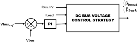
In Figure 3, we present the DC bus voltage regulation strategy.

Download: Download full-size image

Figure 3. DC Bus Voltage Regulation Strategy.

This figure shows a DC bus voltage regulation strategy in this microgrid system. The principle is based on the comparison between the measured voltage of the Vbus bus and its reference value Vbus, ref. The deviation generated is processed by a PI (Proportional-Integral) regulator, which allows to dynamically correct variations and guarantee the stability of the voltage.

Additional input signals, such as the current from the photovoltaic array (Ibus,pv) and the load current (ILoad), are taken into account in order to adapt the control according to the production-consumption balance. This information is sent to the DC Bus Voltage Control Strategy block, which generates control signals denoted as βboost and βbuck.

These coefficients correspond respectively to the boost and buck modes of the bidirectional converter, thus ensuring optimal regulation of the DC bus voltage despite fluctuations in load or renewable production.

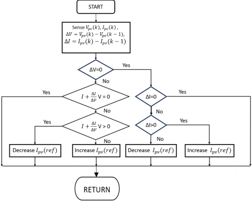
(iii). MPPT Increment

In Figure 4, we present the Maximum Power Point Tracking (MPPT) algorithm based on the Incremental Conductance method

[22, 23]

With each iteration, the system measures the voltage

V_{pv} (k)

and the current

I_{pv} (k)

delivered by the photovoltaic array, then calculates the instantaneous variations

Δ V = V_{pv} (k) - V_{pv} (k - 1)

Δ I = I_{pv} (k) - I_{pv} (k - 1)

. These two quantities allow us to evaluate the discrete derivative of power with respect to voltage:

\frac{dP}{dV} = I + V \frac{dI}{dV} \approx I + V \frac{Δ I}{Δ V} .

(7)

The operating condition at the maximum power point (MPP) is reached when

\frac{dP}{dV} = 0

, that is, when the instantanous conductance

I / V

is equal to the incremental conductance

Δ I / Δ V

The algorithm compares these two conductances to dynamically adjust the reference current setpoint

I_{pvref}

1) If

I / V < - Δ I / Δ V

, the system is to the left of the MPP and the algorithm is increasing

I_{pv} (ref)

to move the operating point to a higher voltage.

2) If

I / V > - Δ I / Δ V

, the system is to the right of the MPP and

I_{pv} (ref)

is decreased in order to reduce the operating voltage.

3) Finally, when

I / V = - Δ I / Δ V

, the generator operates at its maximum power point, and no change in

I_{pv} (ref)

is carried out.

The decision-making scheme presented also handles special cases where

Δ V = 0

Δ I = 0

, to avoid dividing by zero and to maintain tracking stability. This approach provides real-time adaptive control of the operating point, allowing for better tracking accuracy and increased responsiveness to rapid irradiance and temperature variations, while limiting oscillations around the MPP.

Download: Download full-size image

Figure 4. The incremental conductance algorithm.

(iv). Energy Management

The EMS is the decision-making level. It receives the measured quantities (PV power

P_{pv}

, power consumption

P_{load}

, battery SoC, bus voltage) and calculates the power sharing instructions according to a pre-established strategy (prioritization of PV energy, maintenance of bus voltage, battery fallback if deficit, battery recharge in case of surplus). Decision rules can be formulated by deterministic logics (thresholds and priorities), optimizing strategies (cost minimization or maximization of self-consumption) or predictive approaches. The outputs of the EMS are power/current commands transmitted to the converters' control loops.

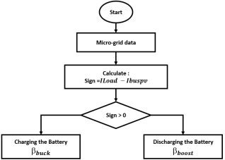
In Figure 5, we present the energy management algorithm in a micro-PV-battery grid.

Download: Download full-size image

Figure 5. Energy management algorithm in a micro-PV-battery grid.

The algorithm shown in Figure 5 shows the energy management strategy adopted within the photovoltaic micro-grid integrating a battery storage system. The objective of this decision-making logic is to ensure the dynamic balance between the power produced by the photovoltaic array and the power demanded by the load, while optimizing the use of the battery.

First, the data from the system is acquired, namely the current supplied by the photovoltaic array (Ibuspv) and the current demanded by the load (ILoad). From these metrics, a decision variable denoted Sign is computed according to the following relationship:

Sign=

ILoad - Ibuspv

This variable is used to determine the energy state of the system:

If Sign>0, The demand of the load is higher than the photovoltaic production. The energy deficit is then compensated by discharging the battery via a voltage step-up converter (Boost).

If Sign<0, photovoltaic production exceeds demand. The excess is stored in the battery through a step-down converter (Buck).

The Sign=0 case corresponds to a situation of perfect equilibrium between production and demand, in which the battery does not intervene.

Thus, the algorithm ensures adaptive and autonomous energy management, allowing both the continuity of the load supply and the maximum recovery of the available solar energy. In addition, the use of suitable DC/DC converters (Buck or Boost) ensures efficient energy transfer and helps to preserve battery life.

3. Case Study

3.1. Presentation of the Study Area

The site chosen for the study is Gandon, a rural community located in northwestern Senegal, in the department of Saint-Louis. It is bordered to the northwest by the Senegal River and the Atlantic Ocean. The geographical coordinates of the site are 15.96° North, 16.45° West

[24]

(Figure 6).

Download: Download full-size image

Figure 6. Location of the site

[24]

3.2. Weather Data

Between 1994 and 2018, the average solar irradiance in Saint-Louis was 5.88 kWh/m²/day and 2154 kWh/m²/year

[25]

, while measurements carried out in Gandon between June 2004 and May 2005 indicated 5.61 kWh/m²/day

[26]

. These data measured during this period were used in this study.

3.3. Load and Daily Power Profile

Figure 7 shows the hourly profile of the power of consumption loads and pumping (Ppump) on a typical day in a rural village in West Africa. This profile reflects the water requirements for domestic uses, irrigation, and sometimes livestock watering, as well as the energy consumption of auxiliary loads.

Download: Download full-size image

Figure 7. Hourly profile of the power of consumption loads in a village in West Africa.

In Figure 8, we present the daily profile of the power delivered by the micro-grid.

Download: Download full-size image

Figure 8. Daily profile of the power delivered by the micro-grid.

Figure 8 shows the hourly evolution of the power supplied by the micro-grid on a representative day. The profile shows a low baseline consumption (≤ 3 kW) during the night and morning, followed by a first moderate rise around 6 a.m.

(≈ 7 kW). Charging then remained almost stable at an average level until the end of the afternoon, before peaking at around 18–19 h, reaching around 31 kW. This maximum reflects the strong residential demand in the evening. Finally, the power gradually decreases to values below 5 kW at the end of the day.

4. Results and Discussion

The simulation results obtained under overcast and clear skies make it possible to evaluate the performance of the PV-battery system in a rural microgrid with agricultural pumping. The analysis focuses on the evolution of currents, voltages, powers and the state of charge (SOC), in order to highlight the impact of sunlight conditions on the stability of the DC bus, storage management and power continuity.

4.1. Overcast Scenario

Analysis of the evolution of the photovoltaic current and the setpoint

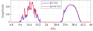
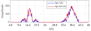
In order to analyze the performance of the MPPT algorithm under overcast conditions, Figure 9 represents the evolution of the measured PV current (Ipv) and the setpoint (Ipvref) over 48 h, covering two consecutive days.

Download: Download full-size image

Figure 9. Evolution of the real photovoltaic current (Ipv) and the setpoint (Ipvref).

Under the overcast sky, the photovoltaic current Ipv (blue) closely follows the reference set Ipvref (red). Two daily cycles are observed (≈14 h and ≈38 h), corresponding to the peaks of solar irradiation. The maximum amplitude reaches about 200 A, reflecting good operation of the PV generator. The point deviations between Ipv and Ipvref remain limited and less than 5%, confirming the performance of the MPPT algorithm to ensure fast and accurate monitoring of the setpoint, even during rapid fluctuations due to cloudy passages. The symmetry between the two cycles indicates a reproducibility of the system's behavior over several days. These results validate the efficiency of the regulation in terms of robustness and stability, which are essential to ensure continuous and reliable energy production in the context of rural microgrids and agricultural pumping applications.

Analysis of the current evolution of the PV bus

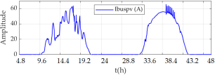
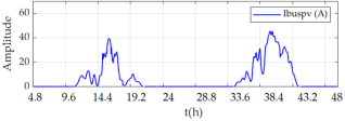
In order to evaluate the dynamics of the DC bus, Figure 10 presents the evolution of the PV bus current (Ibuspv) over 48 h, allowing to analyze the impact of solar variability on the energy injected and the stability of the system.

Download: Download full-size image

Figure 10. PV bus current (Ibuspv).

Figure 10 shows the evolution of the photovoltaic bus (Ibuspv) power over a 48-hour window. Two distinct daily cycles are observed, with maximum amplitudes of the order of 40 A on the first day and slightly higher (≈45 A) on the second. The rapid fluctuations around the peaks reflect the effect of cloud passages, confirming the DC bus's strong dependence on incident irradiance. This daily variability conditions the energy actually available for storage and pumping, highlighting the need for a robust energy management strategy to maintain continuity of service.

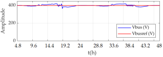
Relationship between DC bus voltage and setpoint

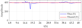
Figure 11 shows the evolution of the DC bus voltage (Vbus) as well as the control setpoint (Vbusref) over a period of 48 hours. The objective is to evaluate the stability of the control under variable conditions, especially in the face of fluctuations in the environment or loads.

Download: Download full-size image

Figure 11. Evolution of the DC bus voltage and the setpoint.

The bus voltage (Vbus) (Figure 11) remains generally around the set point set at 400 V, which attests to a good stability of the regulation over the period observed. However, there are occasional disturbances, particularly around t ≈ 5 p.m., when a sudden drop in voltage to about 250V is observed before a rapid return to the nominal value. This dip likely reflects a rapid change in operating conditions, such as a sudden drop in PV generation or a momentary load on the grid. Another more moderate disturbance is perceptible around t ≈ 39 h, with smaller deviations around the setpoint. Despite these events, the control ensures an effective correction of deviations, thus guaranteeing the continuity of the power supply. These results underline the robustness of the control system, while suggesting the interest of integrating smoothing or storage devices to mitigate the effects of fast transients.

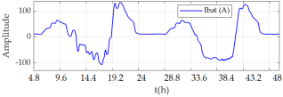
Analysis of battery current and battery bus curves

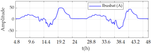
In order to analyze the energy behavior of the storage system, the figure below shows the evolution of the current flowing through the battery (Ibat) as well as the current flowing between the DC bus and the battery (Ibusbat) over a period of 48 hours under overcast conditions.

a) Evolution of the battery current as a function of time

Download: Download full-size image

a) Evolution of the battery current as a function of time

b) Evolution of the current flowing between the DC bus and the battery

Download: Download full-size image

Figure 12. Evolution of Ibat and Ibusbat.

The first curve (Figure 12) is represented the evolution of the Ibat battery current over a period of 48 hours in a pumping site supplied by a photovoltaic micro-grid. The amplitude of the current varies between +100 A (charging phase) and –100 A (discharge phase), reflecting a marked alternation between the accumulation of solar energy and its release to meet the demand of the pumping system. The profile of Ibat reveals well-defined daily cycles, with significant peaks around t ≈ 7 p.m. and t ≈ 42 h, corresponding to periods of high pumping or episodes of irregular sunshine.

The second curve shows the Ibusbat current, representing the energy exchanges between the DC bus and the battery. This current has a reduced amplitude, around ±60 A, and follows a dynamic similar to that of Ibat, with more attenuated variations. This highlights the role of the DC bus as a buffer interface, absorbing or supplying energy depending on the state of the system, while ensuring a stable power supply to the pump motor.

These results confirm the PV-battery system's ability to adapt to rapidly changing climatic conditions and fluctuations in hydraulic demand. They also highlight the importance of an optimized energy management strategy to ensure continuity of power, limit excessive stress on the battery, and thus extend its life.

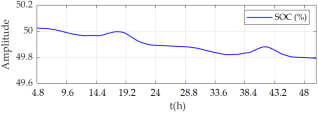
After analyzing the battery charge and discharge currents (Ibat) as well as the energy exchanges with the DC bus (Ibusbat), it is relevant to examine the impact of these flows on the overall state of charge of the system. For this purpose, Figure 13 shows the evolution of the battery's State of Charge (SOC) over a period of 48 hours.

Download: Download full-size image

Figure 13. Evolution of the battery's state of charge (SOC).

Figure 13 shows the change in the battery state of charge (SOC) expressed as a percentage, over a 48-hour period. There is a relatively small variation in the SOC, ranging from 50% to 49.7%, indicating a quasi-steady state operation of the storage system.

This low amplitude of variation in the SOC reflects an overall balance between the charge and discharge phases, suggesting that the battery operates in a restricted operating area, in order to preserve its lifespan and minimize deep cycling. The slightly decreasing trend in SOC over the entire period could result from energy demand slightly higher than PV production, or from an overall system efficiency slightly lower than the unit.

Slight changes in the profile, visible in particular around t ≈ 7 p.m. and t ≈ 42 h, coincide with the fluctuations observed on the Ibat and Ibusbat currents, confirming the impact of charge/discharge variations on the instantaneous state of charge.

These results underline the importance of fine-grained energy management in PV-battery systems, especially in the context of solar pumping, where continuity of service is highly dependent on the ability of the storage to maintain an optimal level of SOC despite variations in production and demand.

Battery Voltage Variation (Vbat) Analysis:

After the analysis of the currents and the state of charge, Figure 14 shows the temporal evolution of the battery voltage (Vbat) over a period of 48 hours.

Download: Download full-size image

Figure 14. Variation of battery voltage (Vbat).

Figure 14 shows the variation in battery voltage (Vbat) between about 195 V and 208 V over 48 hours, reflecting the charge and discharge cycles related to the dynamics of the solar pumping system. The voltage drops observed around t ≈ 7 p.m. and t ≈ 43 h correspond to larger discharge phases, while the increases around t ≈ 3 p.m. and t ≈ 38 h coincide with recharging periods, in connection with photovoltaic energy availability.

The voltage remains overall close to 200 V outside of peaks, indicating effective control of the energy management system, ensuring storage stability and safety. Vbat's moderate modulation helps to limit the premature aging of batteries. This evolution is consistent with the current and state of charge profiles, confirming the good interaction between production, storage and consumption in this microgrid.

Analysis of power flows in the solar pumping system:

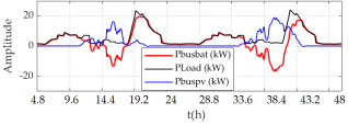
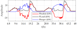
Figure 15 shows the evolution of the PV (Pbuspv), charge (PLoad) and battery (Pbusbat) powers over a 48-hour period in a solar pumping system.

Download: Download full-size image

Figure 15. Pbuspv (PV), PLoad (charging) and Pbusbat (battery) powers in kW.

Figure 15 shows the temporal evolution over 48 hours of three key powers in the system: the power injected or taken by the battery via the DC bus (Pbusbat, in red), the charging power of the system (PLoad, in black), and the power produced by the photovoltaic panels (Pbuspv, in blue).

It can be observed that photovoltaic power (Pbuspv) shows significant peaks during the daytime periods, in particular between t ≈ 9 a.m. and 6 p.m. and between t ≈ 35 a.m. and 43 p.m., which corresponds to the hours of maximum sunshine. Outside these ranges, PV production is almost zero, indicating the absence of solar irradiation.

The charging power (PLoad) shows profiles corresponding to the energy needs of the pumping system, with peaks largely coinciding with those of solar production, but also significant consumption during the night (PLoad > 0 while Pbuspv ≈ 0), which implies battery power.

The battery power (Pbusbat) oscillates between positive and negative values, indicating the phases of charge (positive power) and discharge (negative power) respectively. For example, during peaks in PV production, Pbusbat is positive, reflecting a recharge of the battery with excess energy. Conversely, when the load is sustained while PV production is low or zero (especially in the evening or early morning), Pbusbat becomes negative, indicating the discharge of the battery to power the charge.

Notably, around t ≈ 7 p.m. and t ≈ 42 h, there are marked fluctuations with rapid transitions between load and discharge, reflecting the dynamic response of the system to variations in demand and production. These cycles underline the importance of fine-grained and responsive energy management to ensure continuity of service and optimize battery life.

This figure highlights the central role of the battery as an energy buffer between the intermittent production of photovoltaics and the variable demand of the pumping system, ensuring a dynamic balance between injection and withdrawal of energy on the DC bus.

4.2. Clear Sky Scenario

In this part, we have analyzed the performance of the PV-battery system in clear sky conditions.

Analysis of the evolution of the photovoltaic current and the setpoint

In order to evaluate the performance of the MPPT control applied to the photovoltaic array, Figure 16 shows the comparison between the measured PV current (Ipv) and its reference current (Ipvref) over a 48-hour period.

Download: Download full-size image

Figure 16. Evolution of the real photovoltaic current (Ipv) and the setpoint (Ipvref).

Figure 16 shows the temporal evolution of the current delivered by the photovoltaic array (Ipv, in blue) and the associated reference current (Ipvref, in red) over a period of 48 hours. These curves are used to evaluate the performance of the Maximum Power Point Tracking (MPPT) controller.

It can be observed that during the sunlight phases (≈ 9 a.m. to 7 p.m. and ≈ 33 p.m. to 43 p.m.), Ipv closely follows Ipvref, reflecting a good accuracy of the MPPT control. Rapid variations of Ipvref, particularly visible between 12 and 18 h, are effectively monitored by Ipv, despite the presence of fluctuations related to system dynamics or rapid irradiance perturbations.

The gap between the two curves remains small overall, indicating that the controller manages to quickly adjust the operating point of the PV array in response to variations in sunlight. The adequacy between Ipv and Ipvref thus confirms the robustness and responsiveness of the control strategy implemented. In the absence of irradiation (t < 9 a.m., t ≈ 7 p.m. to 33 p.m., and t > 43 h), the two currents cancel each other out, as expected.

Analysis of the current evolution of the PV bus

Figure 17 shows the current injected into the DC bus by the photovoltaic array (Ibuspv), highlighting the solar production profiles over a 48-hour period.

Download: Download full-size image

Figure 17. PV bus current (Ibuspv).

Figure 17 shows the current injected on the DC bus (Ibuspv) by the photovoltaic array over 48 hours, under clear sky conditions. The observed profile, with gradual increases in the morning, plateaus in the middle of the day, then decreases in the late afternoon (≈ 9–19 h and ≈ 33–43 h), is characteristic of stable and regular solar production.

The current peaks at about 60 A, indicating operation close to the point of maximum power. The absence of major disturbances or sudden fluctuations confirms the good performance of the system in terms of regulation and injection. The slight oscillations observed around t ≈ 38.5 h remain limited and do not alter the overall stability. This behavior validates the effectiveness of the PV system and its control under optimal conditions.

Relationship between DC bus voltage and setpoint

Figure 18 is used to evaluate the voltage stability of the DC bus by comparing the measured voltage (Vbus) to its reference (Vbusref) over 48 hours of operation.

Download: Download full-size image

Figure 18. Evolution of the DC bus voltage and the setpoint.

Figure 18 shows the evolution of the DC bus voltage (Vbus, in blue) compared to its reference set point (Vbusref, in red) over a period of 48 hours. This figure makes it possible to evaluate the ability of the conversion system to maintain a stable voltage, an essential condition for the proper functioning of the connected equipment.

It can be seen that Vbus closely follows the set point of about 400 V, with small point deviations. Slight ripples appear around t ≈ 6 p.m. and t ≈ 38.5 h, corresponding to rapid changes in PV load or production. However, these fluctuations remain contained, which testifies to the good dynamic stability of the voltage regulator. Overall, the bus voltage is precisely maintained around its set value, which confirms the effectiveness of the control system under normal operating conditions.

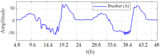
Analysis of battery current and battery bus curves

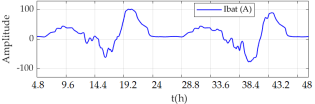
In Figure 19, we present the evolution of the battery current (Ibatt) as well as the current exchanged with the DC bus (Ibusbat), allowing us to analyze the charging and discharging phases over 48 hours of operation.

a) Evolution of the battery as a function of time

Download: Download full-size image

a) Evolution of the battery as a function of time

b) Evolution of the current flowing between the DC bus and the battery

Download: Download full-size image

Figure 19. Evolution of the battery current and the current exchanged between the battery and the DC bus.

Figure 19 shows the evolution of the battery current (Ibatt) and the current exchanged between the battery and the DC bus (Ibusbat) over a period of 48 hours. These two quantities make it possible to evaluate the charge/discharge dynamics of the battery as well as its interaction with the rest of the system.

The Ibatt current (upper figure) shows clear alternations between positive values (charge phase) and negative values (discharge phase). The positive peaks observed around t ≈ 7 p.m. and t ≈ 43 a.m. reflect phases of intense recharging, generally synchronized with peaks in photovoltaic production. Conversely, the discharge phases (negative current) appear in the evening and during the night, especially around t ≈ 14–18 h and t ≈ 38 h, when the battery compensates for the lack of solar production.

The Ibusbat current (lower figure), representing the current actually injected or taken by the battery on the DC bus, follows the same dynamics as Ibatt, with smaller amplitudes. This is due to internal conversions and possible losses in the power stages. There is a temporal coherence between the two curves, with simultaneous charge/discharge transitions.

The rapid changes visible around t ≈ 38.5 h indicate a dynamic response of the system to fluctuations in load or production. The absence of major instabilities confirms an efficient management of the stored energy. These curves highlight the central role of the battery in the energy balancing of the system, ensuring continuity of service despite the intermittency of the photovoltaic source.

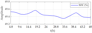
After analyzing the charging and discharging currents of the battery (Ibat) as well as the energy exchanges with the DC bus (Ibusbat), we present in Figure 20, the evolution of the State of Charge (SOC) of the battery over a period of 48 hours.

Download: Download full-size image

Figure 20. Evolution of the battery's state of charge (SOC).

Figure 20 shows the evolution of the battery's State of Charge (SOC) over a period of 48 hours. The SOC remains overall around 49.4% to 49.6%, with small daily variations. These small oscillations reflect an energy balance between the load phases (during periods of high photovoltaic production) and the discharge phases (when the system load is sustained and solar production is absent). The stability of the SOC in this restricted range confirms efficient energy management, avoiding both overload and deep discharge. This behaviour indicates that the control strategy ensures operation in a quasi-steady state, with moderate stress on the battery, which is favourable to its longevity.

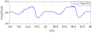
Battery Voltage Variation (Vbat) Analysis:

In Figure 21, we observe the evolution of the battery voltage (Vbat), allowing us to evaluate the impact of the charge and discharge cycles over a period of 48 hours.

Download: Download full-size image

Figure 21. Variation of battery voltage (Vbat).

Figure 21 shows the change in battery voltage (Vbat) over a 48-hour period. It can be observed that Vbat evolves between 195 V and 208 V, reflecting the successive cycles of charge and discharge.

The voltage increases, which can be seen in particular around t ≈ 14–18 h and t ≈ 34–38 h, correspond to charging phases, generally synchronised with photovoltaic production. Conversely, the voltage drops observed around t ≈ 7 p.m. and t ≈ 42 a.m. reflect more sustained periods of discharge, in the absence of solar production. Despite these variations, the voltage remains within a controlled operational range, with no critical overload or undervoltage, which confirms efficient storage management and good battery sizing. The rapid ripples observed around t ≈ 38.5 h are related to fast charge/discharge transients, but do not compromise the overall stability of the system.

Analysis of power flows in the solar pumping system:

Download: Download full-size image

Figure 22. Pbuspv (PV), PLoad (charging) and Pbusbat (battery) powers in Kw.

In Figure 22, we observe the evolution of the key powers in the hybrid system over a period of 48 hours: the power injected or taken by the battery (Pbusbat, in red), the power consumed by the load (PLoad, in black), and the power produced by the photovoltaic array (Pbuspv, in blue).

PV production (Pbuspv) has two active periods, between t ≈ 9–19 h and t ≈ 33–43 h, corresponding to the hours of sunshine. Production peaks partly coincide with peak loads, but are not always sufficient to cover demand, especially during consumption peaks in the evening.

The battery plays a buffering role: Pbusbat is positive when the battery is charged (excess PV production), and negative when it is used to power the load in the absence of solar production. The rapid transitions around t ≈ 7 p.m. and t ≈ 42 h. illustrate the dynamic response of the system to simultaneous variations in production and demand. These curves confirm a reactive and balanced energy management, ensuring continuity of service while making the most of the intermittency of the photovoltaic source.

5. Conclusion

The analysis of the two operating scenarios, under clear skies and overcast skies, demonstrates that the proposed photovoltaic system with storage ensures a reliable and robust response to the energy and water needs of rural areas. Thanks to the combination of InC-type MPPT monitoring, PI regulation and a coordinated energy management strategy, the architecture studied guarantees both the supply of electricity for domestic uses and irrigation, while maintaining the stability of the DC bus and the autonomy of the batteries. These results confirm the relevance of the scheme developed as a sustainable and adaptable solution to the varied climatic contexts encountered in sub-Saharan Africa. For future work, it would be interesting to integrate a complementary wind source and develop another type of converter to improve the flexibility and efficiency of the system.

Abbreviations

AC	Alternating current
DC	Direct current
EMF	Electromotive Force
EMS	Energy Management System
MPPT	Maximum Power Point Tracking
PI	Proportional-Integral regulator
PV	Photovoltaic
SOC	State of Charge

Author Contributions

Souleymane Soumah: Conceptualization, Methodology, Resources, Writing – original draft, Writing – review & editing

Mouhamadou Falilou Ndiaye: Formal Analysis, Project administration, Validation, Visualization

Mohamed Ansoumane Camara: Formal Analysis, Resources, Visualization

Vincent Sambou: Supervision

Conflicts of Interest

The authors declare no conflicts of interest.

References

[1]	S. C. Bhattacharyya et D. Palit, «A critical review of literature on the nexus between central grid and off-grid solutions for expanding access to electricity in Sub-Saharan Africa and South Asia», Renew. Sustain. Energy Rev., vol. 141, p. 110792, mai 2021, https://doi.org/10.1016/j.rser.2021.110792
[2]	K. M. S. Domegni et Y. O. Azouma, «Productive uses of energy: A solution for promoting energy justice in rural areas in West Africa», Renew. Sustain. Energy Rev., vol. 160, p. 112298, mai 2022, https://doi.org/10.1016/j.rser.2022.112298
[3]	T. Mosetlhe, A. Yusuff, T. Ayodele, et A. Ogunjuyigbe, « Sustainable rural electrification through micro-grids in developing nations — A review of recent development », Energy Rep., vol. 13, p. 1171‑1177, juin 2025, https://doi.org/10.1016/j.egyr.2024.11.040
[4]	A. S. Ba, “Universal and sustainable access to electricity in Senegal: Conditions for success,” Working paper, 2018. RePEc: hal-wpaper: hal-01956217. Available: https://hal.science/hal-01956217v1
[5]	S. Lai, Y. Jia, L. L. Lai, Z. Xu, M. D. McCulloch, et K. P. Wong, «A comprehensive review on large-scale photovoltaic system with applications of electrical energy storage», Renew. Sustain. Energy Rev., vol. 78, p. 439‑451, oct. 2017, https://doi.org/10.1016/j.rser.2017.04.078
[6]	M. Elizabeth Lesala et P. Mukumba, «Hybrid Mini-Grid Solutions to Rural Energy Poverty: Toward Sustainable Energy Access and Socioeconomic Impacts in the Upper Blinkwater Community, South Africa», in Sustainable Development, vol. 34, M. Noguchi, Ed., IntechOpen, 2025. https://doi.org/10.5772/intechopen.1009217
[7]	N. Lefore, A. Closas, et P. Schmitter, «Solar for all: A framework to deliver inclusive and environmentally sustainable solar irrigation for smallholder agriculture», Energy Policy, vol. 154, p. 112313, juill. 2021, https://doi.org/10.1016/j.enpol.2021.112313
[8]	L. Richard, D. Frey, M.-C. Alvarez-Herault, et B. Raison, «A Decentralized and Communication-free Control Algorithm of DC Microgrids for the Electriﬁcation of Rural Africa»." 2022 24th European Conference on Power Electronics and Applications (EPE'22 ECCE Europe), Hanover, Germany, 2022, pp. 1-10. Available: https://www.researchgate.net/publication/374294846
[9]	R. J. J. Molu, S. Raoul Dzonde Naoussi, P. Wira, W. F. Mbasso, S. T. Kenfack, et S. Kamel, «Optimization-based energy management system for grid-connected photovoltaic/battery microgrids under uncertainty», Case Stud. Chem. Environ. Eng., vol. 8, p. 100464, dec. 2023, https://doi.org/10.1016/j.cscee.2023.100464
[10]	O. Cisse, M. F. Ndiaye, and P. A. Ndiaye, “Energy management of a photovoltaic / wind / battery pumping system on a farm,” Afrique SCIENCE, vol. 14, no. 1, pp. 292–303, 2018. Available: https://www.afriquescience.net/admin/postpdfs/a3da4439a929ede95978e35a9bc9845c1729716035.pdf
[11]	M. Rumbayan, I. Pundoko, S. R. Sompie, and D. G. Ruindungan, «Integration of smart water management and photovoltaic pumping system to supply domestic water for rural communities», Results Eng., vol. 25, p. 103966, mars 2025, https://doi.org/10.1016/j.rineng.2025.103966
[12]	R. Sayani, P. O. Arriaga, P. Sandwell and al., «Sizing solar-based mini-grids for growing electricity demand: Insights from rural India», J. Phys. Energy, vol. 5, n^o 1, p. 014004, janv. 2023, https://doi.org/10.1088/2515-7655/ac9dc0
[13]	G. Kyriakarakos, A. T. Balafoutis, et D. Bochtis, «Proposing a Paradigm Shift in Rural Electrification Investments in Sub-Saharan Africa through Agriculture», Sustainability, vol. 12, no 8, p. 3096, avr. 2020, https://doi.org/10.3390/su12083096
[14]	T. Liu and al., «A Novel Simulation Method for Analyzing Diode Electrical Characteristics Based on Neural Networks», Electronics, vol. 10, no 19, p. 2337, sept. 2021, https://doi.org/10.3390/electronics10192337
[15]	Z. Song and al., «An Effective Method to Accurately Extract the Parameters of Single Diode Model of Solar Cells», Nanomaterials, vol. 11, no 10, p. 2615, oct. 2021, https://doi.org/10.3390/nano11102615
[16]	X. Zhang, J. Hou, Z. Wang, et Y. Jiang, «Study of SOC Estimation by the Ampere-Hour Integral Method with Capacity Correction Based on LSTM», Batteries, vol. 8, no 10, p. 170, oct. 2022, https://doi.org/10.3390/batteries8100170
[17]	M. B. Camara, H. Gualous, F. Gustin, A. Berthon, et B. Dakyo, «DC/DC Converter Design for Supercapacitor and Battery Power Management in Hybrid Vehicle Applications—Polynomial Control Strategy», IEEE Trans. Ind. Electron., vol. 57, no 2, p. 587‑597, févr. 2010, https://doi.org/10.1109/TIE.2009.2025283
[18]	L. Chen and al., «Estimation the internal resistance of lithium-ion-battery using a multi-factor dynamic internal resistance model with an error compensation strategy», Energy Reports, vol. 7, p. 3050‑3059, nov. 2021, https://doi.org/10.1016/j.egyr.2021.05.027
[19]	S. Xie, X. Zhang, W. Bai, A. Guo, W. Li, et R. Wang, «State‐of‐Charge Estimation of Lithium‐Ion Battery Based on an Improved Dual‐Polarization Model», Energy Tech, vol. 11, no 4, p. 2201364, avr. 2023, https://doi.org/10.1002/ente.202201364
[20]	Y. Wang and al., «A comprehensive review of battery modeling and state estimation approaches for advanced battery management systems», Renewable and Sustainable Energy Reviews, vol. 131, p. 110015, oct. 2020, https://doi.org/10.1016/j.rser.2020.110015
[21]	C. B. Nzoundja Fapi, M. L. Touré, M.-B. Camara, et B. Dakyo, «Control Strategy for DC Micro-Grids in Heat Pump Applications with Renewable Integration», Electronics, vol. 14, no 1, p. 150, janv. 2025, https://doi.org/10.3390/electronics14010150
[22]	«Hybrid, optimization, intelligent and classical PV MPPT techniques: Review», CSEE JPES, 2020, https://doi.org/10.17775/CSEEJPES.2019.02720
[23]	R. B. Bollipo, S. Mikkili, et P. K. Bonthagorla, « Critical Review on PV MPPT Techniques: Classical, Intelligent and Optimisation », IET Renewable Power Gen, vol. 14, no 9, p. 1433‑1452, juill. 2020, https://doi.org/10.1049/iet-rpg.2019.1163
[24]	D. F, T. A. K., and B. L, «THE SILTING UP OF VEGETABLE CROP AREA IN GANDIOLAIS (NORTHERN COAST OF SENEGAL)», Int. J. Eng. Sci. Tech, vol. 6, no 3, p. 35‑51, mai 2022, https://doi.org/10.29121/ijoest.v6.i3.2022.246
[25]	Atlas solaire mondial. (Accessed 11 september 2025). Available from: https://globalsolaratlas.info/map?c=11.523088,8.173828,3
[26]	O. Cisse, L. Thiaw, S. Sawadogo, and D. Kobor, «Smart Energy Management of a Stand-Alone PV/Wind System: Application for Rural Agricultural Development».

Cite This Article

Plain Text BibTeX RIS

APA Style

Soumah, S., Ndiaye, M. F., Camara, M. A., Sambou, V. (2025). Energy Management of PV-Battery Systems for Rural Microgrids and Agricultural Water Pumping Applications in Senegal. Science Journal of Energy Engineering, 13(4), 192-205. https://doi.org/10.11648/j.sjee.20251304.12

Copy | Download

ACS Style

Soumah, S.; Ndiaye, M. F.; Camara, M. A.; Sambou, V. Energy Management of PV-Battery Systems for Rural Microgrids and Agricultural Water Pumping Applications in Senegal. Sci. J. Energy Eng. 2025, 13(4), 192-205. doi: 10.11648/j.sjee.20251304.12

Copy | Download

AMA Style

Soumah S, Ndiaye MF, Camara MA, Sambou V. Energy Management of PV-Battery Systems for Rural Microgrids and Agricultural Water Pumping Applications in Senegal. Sci J Energy Eng. 2025;13(4):192-205. doi: 10.11648/j.sjee.20251304.12

Copy | Download

@article{10.11648/j.sjee.20251304.12,
  author = {Souleymane Soumah and Mouhamadou Falilou Ndiaye and Mohamed Ansoumane Camara and Vincent Sambou},
  title = {Energy Management of PV-Battery Systems for Rural Microgrids and Agricultural Water Pumping Applications in Senegal},
  journal = {Science Journal of Energy Engineering},
  volume = {13},
  number = {4},
  pages = {192-205},
  doi = {10.11648/j.sjee.20251304.12},
  url = {https://doi.org/10.11648/j.sjee.20251304.12},
  eprint = {https://article.sciencepublishinggroup.com/pdf/10.11648.j.sjee.20251304.12},
  abstract = {This work proposes an optimized energy management strategy for a photovoltaic (PV) system coupled with batteries, intended for both rural electrification and agricultural pumping applications. The approach takes into account photovoltaic generation, battery storage and demand management to ensure a balance between domestic needs and irrigation requirements. For the MPPT of PVs with an installed power of 36.6 kWp, we used the conductance increment algorithm (Inc) to provide the PV current reference and the power transfer to the DC bus was provided via a Boost chopper. To ensure the stability of the DC bus voltage, a PI regulator is dimensioned and a management algorithm is developed to control the Buck-Boost coupled to the grid. This algorithm makes it possible to store the excess PV production in the battery pack and to return them in the event of a deficit through the bidirectional converter. In addition, the proposed strategy ensures coordinated operation between generation, storage, and agricultural pumping in order to guarantee the continuity of supply under varying climatic and load conditions. The simulation results highlight the potential of PV-battery microgrids to reduce reliance on diesel, improve access to water for agriculture, and strengthen the sustainability of rural communities. The findings demonstrate that the proposed system achieves stable voltage regulation, efficient energy allocation, and improved autonomy for isolated sites. The study thus proposes a framework that can be replicated in similar contexts in sub-Saharan Africa, simultaneously contributing to energy access and food security.},
 year = {2025}
}

Copy | Download

TY  - JOUR
T1  - Energy Management of PV-Battery Systems for Rural Microgrids and Agricultural Water Pumping Applications in Senegal
AU  - Souleymane Soumah
AU  - Mouhamadou Falilou Ndiaye
AU  - Mohamed Ansoumane Camara
AU  - Vincent Sambou
Y1  - 2025/12/17
PY  - 2025
N1  - https://doi.org/10.11648/j.sjee.20251304.12
DO  - 10.11648/j.sjee.20251304.12
T2  - Science Journal of Energy Engineering
JF  - Science Journal of Energy Engineering
JO  - Science Journal of Energy Engineering
SP  - 192
EP  - 205
PB  - Science Publishing Group
SN  - 2376-8126
UR  - https://doi.org/10.11648/j.sjee.20251304.12
AB  - This work proposes an optimized energy management strategy for a photovoltaic (PV) system coupled with batteries, intended for both rural electrification and agricultural pumping applications. The approach takes into account photovoltaic generation, battery storage and demand management to ensure a balance between domestic needs and irrigation requirements. For the MPPT of PVs with an installed power of 36.6 kWp, we used the conductance increment algorithm (Inc) to provide the PV current reference and the power transfer to the DC bus was provided via a Boost chopper. To ensure the stability of the DC bus voltage, a PI regulator is dimensioned and a management algorithm is developed to control the Buck-Boost coupled to the grid. This algorithm makes it possible to store the excess PV production in the battery pack and to return them in the event of a deficit through the bidirectional converter. In addition, the proposed strategy ensures coordinated operation between generation, storage, and agricultural pumping in order to guarantee the continuity of supply under varying climatic and load conditions. The simulation results highlight the potential of PV-battery microgrids to reduce reliance on diesel, improve access to water for agriculture, and strengthen the sustainability of rural communities. The findings demonstrate that the proposed system achieves stable voltage regulation, efficient energy allocation, and improved autonomy for isolated sites. The study thus proposes a framework that can be replicated in similar contexts in sub-Saharan Africa, simultaneously contributing to energy access and food security.
VL  - 13
IS  - 4
ER  -

Copy | Download

Author Information

Souleymane Soumah

Water, Energy, Environment and Industrial Processes Laboratory (LE3PI), Cheikh Anta Diop University, Dakar, Senegal;Automatic and Energetic Lecturing and Research Laboratory (LENA), Gamal Abdel Nasser University of Conakry, Conakry, Guinea

Contact Email

http://orcid.org/0009-0002-1280-5570
Mouhamadou Falilou Ndiaye

Water, Energy, Environment and Industrial Processes Laboratory (LE3PI), Cheikh Anta Diop University, Dakar, Senegal

Contact Email

http://orcid.org/0000-0002-9421-7598
Mohamed Ansoumane Camara

Automatic and Energetic Lecturing and Research Laboratory (LENA), Gamal Abdel Nasser University of Conakry, Conakry, Guinea

Contact Email

http://orcid.org/0009-0009-0922-3415
Vincent Sambou

Water, Energy, Environment and Industrial Processes Laboratory (LE3PI), Cheikh Anta Diop University, Dakar, Senegal

Contact Email

http://orcid.org/0000-0002-1042-8348

Download PDF

Submit an Article

Plain Text BibTeX RIS

APA Style

Soumah, S., Ndiaye, M. F., Camara, M. A., Sambou, V. (2025). Energy Management of PV-Battery Systems for Rural Microgrids and Agricultural Water Pumping Applications in Senegal. Science Journal of Energy Engineering, 13(4), 192-205. https://doi.org/10.11648/j.sjee.20251304.12

Copy | Download

ACS Style

Soumah, S.; Ndiaye, M. F.; Camara, M. A.; Sambou, V. Energy Management of PV-Battery Systems for Rural Microgrids and Agricultural Water Pumping Applications in Senegal. Sci. J. Energy Eng. 2025, 13(4), 192-205. doi: 10.11648/j.sjee.20251304.12

Copy | Download

AMA Style

Soumah S, Ndiaye MF, Camara MA, Sambou V. Energy Management of PV-Battery Systems for Rural Microgrids and Agricultural Water Pumping Applications in Senegal. Sci J Energy Eng. 2025;13(4):192-205. doi: 10.11648/j.sjee.20251304.12

Copy | Download

@article{10.11648/j.sjee.20251304.12,
  author = {Souleymane Soumah and Mouhamadou Falilou Ndiaye and Mohamed Ansoumane Camara and Vincent Sambou},
  title = {Energy Management of PV-Battery Systems for Rural Microgrids and Agricultural Water Pumping Applications in Senegal},
  journal = {Science Journal of Energy Engineering},
  volume = {13},
  number = {4},
  pages = {192-205},
  doi = {10.11648/j.sjee.20251304.12},
  url = {https://doi.org/10.11648/j.sjee.20251304.12},
  eprint = {https://article.sciencepublishinggroup.com/pdf/10.11648.j.sjee.20251304.12},
  abstract = {This work proposes an optimized energy management strategy for a photovoltaic (PV) system coupled with batteries, intended for both rural electrification and agricultural pumping applications. The approach takes into account photovoltaic generation, battery storage and demand management to ensure a balance between domestic needs and irrigation requirements. For the MPPT of PVs with an installed power of 36.6 kWp, we used the conductance increment algorithm (Inc) to provide the PV current reference and the power transfer to the DC bus was provided via a Boost chopper. To ensure the stability of the DC bus voltage, a PI regulator is dimensioned and a management algorithm is developed to control the Buck-Boost coupled to the grid. This algorithm makes it possible to store the excess PV production in the battery pack and to return them in the event of a deficit through the bidirectional converter. In addition, the proposed strategy ensures coordinated operation between generation, storage, and agricultural pumping in order to guarantee the continuity of supply under varying climatic and load conditions. The simulation results highlight the potential of PV-battery microgrids to reduce reliance on diesel, improve access to water for agriculture, and strengthen the sustainability of rural communities. The findings demonstrate that the proposed system achieves stable voltage regulation, efficient energy allocation, and improved autonomy for isolated sites. The study thus proposes a framework that can be replicated in similar contexts in sub-Saharan Africa, simultaneously contributing to energy access and food security.},
 year = {2025}
}

Copy | Download

TY  - JOUR
T1  - Energy Management of PV-Battery Systems for Rural Microgrids and Agricultural Water Pumping Applications in Senegal
AU  - Souleymane Soumah
AU  - Mouhamadou Falilou Ndiaye
AU  - Mohamed Ansoumane Camara
AU  - Vincent Sambou
Y1  - 2025/12/17
PY  - 2025
N1  - https://doi.org/10.11648/j.sjee.20251304.12
DO  - 10.11648/j.sjee.20251304.12
T2  - Science Journal of Energy Engineering
JF  - Science Journal of Energy Engineering
JO  - Science Journal of Energy Engineering
SP  - 192
EP  - 205
PB  - Science Publishing Group
SN  - 2376-8126
UR  - https://doi.org/10.11648/j.sjee.20251304.12
AB  - This work proposes an optimized energy management strategy for a photovoltaic (PV) system coupled with batteries, intended for both rural electrification and agricultural pumping applications. The approach takes into account photovoltaic generation, battery storage and demand management to ensure a balance between domestic needs and irrigation requirements. For the MPPT of PVs with an installed power of 36.6 kWp, we used the conductance increment algorithm (Inc) to provide the PV current reference and the power transfer to the DC bus was provided via a Boost chopper. To ensure the stability of the DC bus voltage, a PI regulator is dimensioned and a management algorithm is developed to control the Buck-Boost coupled to the grid. This algorithm makes it possible to store the excess PV production in the battery pack and to return them in the event of a deficit through the bidirectional converter. In addition, the proposed strategy ensures coordinated operation between generation, storage, and agricultural pumping in order to guarantee the continuity of supply under varying climatic and load conditions. The simulation results highlight the potential of PV-battery microgrids to reduce reliance on diesel, improve access to water for agriculture, and strengthen the sustainability of rural communities. The findings demonstrate that the proposed system achieves stable voltage regulation, efficient energy allocation, and improved autonomy for isolated sites. The study thus proposes a framework that can be replicated in similar contexts in sub-Saharan Africa, simultaneously contributing to energy access and food security.
VL  - 13
IS  - 4
ER  -

Copy | Download